Navigating the financial markets can feel like a roller coaster, with its ups and downs, twists and turns. Understanding how volatility behaves over time is crucial. the Autoregressive Conditional Heteroskedasticity (ARCH) model — a powerful tool that can transform the way you view market fluctuations. This article is here to break down the ARCH model in simple terms, show you its key parts, and explain what it means for investment decisions. We’ll also dive into real-world examples using data straight from Yahoo Finance, so you can see it in action. Ready to demystify market volatility? Let’s get started! Here are the focus topics I will discuss related to Arch Models.

Table of Contents

Key Components of the ARCH Model

Real-World Examples

What are the Investment implications?

Conclusion

Key Components of the ARCH Model

Mean Model (mu):

• Represents the average return of the time series.
• A significant mu suggests a consistent average return, while a non-significant mu indicates the mean return is not statistically different from zero.

Volatility Model:

• Baseline Volatility (omega): The constant term in the volatility equation. A positive and significant omega indicates inherent variability in the series that persists over time, irrespective of market shocks.
• Impact of Past Volatility (alpha): Coefficients that measure the influence of past squared residuals (past volatility) on current volatility. Significant alpha values suggest that past volatility affects current volatility, indicating volatility clustering.

The data used in this article was sourced from Yahoo Finance, covering the period from May 1, 2010, to January 1, 2023. The financial instruments analysed include the ^FTSE index and BTC-USD (Bitcoin). The time series data were processed and examined by the author using Python.

Now, let’s bring the ARCH model to life with some real-world examples. We’ll see how this powerful tool works by diving into the volatility patterns of the ^FTSE index and Bitcoin (BTC-USD). Buckle up, because it’s time to explore the dynamic world of financial volatility!

Real-World Examples

^FTSE index Arch Model summary

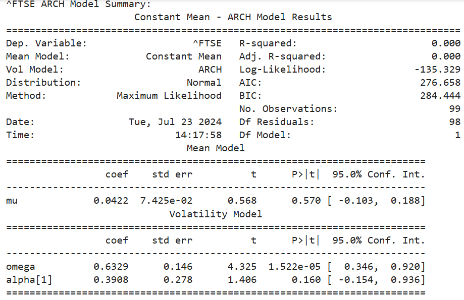
• Mean Model (mu): The mu value of 0.0422 is not statistically significant (p-value = 0.570), indicating that the average return of the ^FTSE index is not significantly different from zero. This means there is no reliable trend in the average returns of the index.
• Volatility Model:
• Baseline Volatility (omega): The omega coefficient is positive (0.6329) and statistically significant (p-value = 1.522e-05). This indicates a significant inherent level of volatility in the ^FTSE index, independent of past volatility. For investors, this means there is always some level of risk or uncertainty present, regardless of market conditions.
• Impact of Past Volatility (alpha[1]): The alpha[1] coefficient (0.3908) is not statistically significant (p-value = 0.160). This suggests that past volatility does not significantly influence current volatility in the ^FTSE index. This implies that volatility does not cluster, and high volatility today does not necessarily imply high volatility tomorrow.

Let’s take a look at BTC-USD Arch Model summary

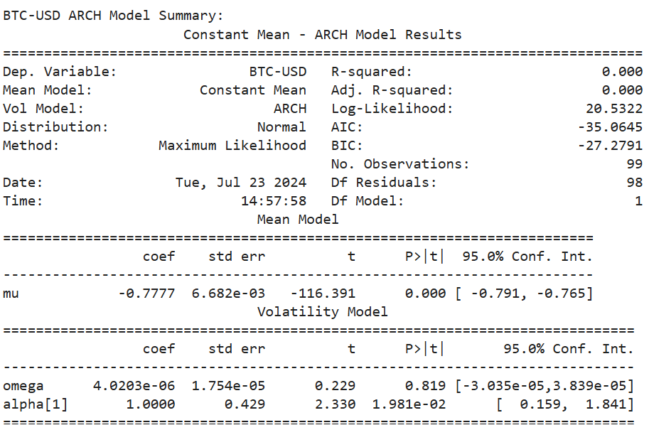
• Mean Model (mu): The mu value of -0.7777 is statistically significant (p-value = 0.000), indicating a consistent average return that is negative. this suggests that Bitcoin, on average, decreased over the period analysed.
• Volatility Model:
• Baseline Volatility (omega): The omega coefficient is positive (4.0203e-06) but not statistically significant (p-value = 0.819). This indicates that the inherent level of volatility is not significantly different from zero, implying that the baseline level of risk is negligible.
• Impact of Past Volatility (alpha[1]): The alpha[1] coefficient is 1.0000 and statistically significant (p-value = 0.0198). This suggests that past volatility significantly influences current volatility in Bitcoin, indicating strong volatility clustering. For investors, this means that periods of high volatility are likely to be followed by high volatility, and low volatility periods are followed by low volatility.

What are the Investment implications?

Inherent Volatility:

• A significant omega value indicates an inherent level of volatility. Investors should account for this baseline risk when making investment decisions. In the BTC-USD example, the insignificant omega value suggests that there is no notable baseline risk, indicating that inherent volatility is negligible. However, in other assets like ^FTSE index example, a significant omega would imply an inherent level of risk that persists regardless of market conditions. Investors should always check the significance of omega to understand the baseline risk.

Volatility Prediction:

• When alpha coefficients are significant, it implies volatility clustering. High volatility today can lead to high volatility tomorrow, which is crucial for predicting future risk. However, an insignificant alpha value indicates a lack of predictability in volatility patterns, making it harder to forecast future volatility based on past data.

Risk Management:

• Strategies should be dynamic and adaptable. Traditional models relying on past volatility patterns may not be effective for all assets. Investors should diversify across different asset classes or sectors to manage risk effectively.

Conclusion

Understanding the ARCH model provides valuable insights into the volatility dynamics of financial time series data. By examining omega and alpha coefficients, investors can better understand inherent risks and volatility patterns. Whether for academic purposes or practical investment strategies, mastering the ARCH model is essential for navigating financial markets effectively.

Note :

This article is provided by Cynthia and it is related to educational purposes. Thanks